Introduction to Bilevel Optimization

It is well known that, without loss of generality, an optimization problem can be defined as finding the set:

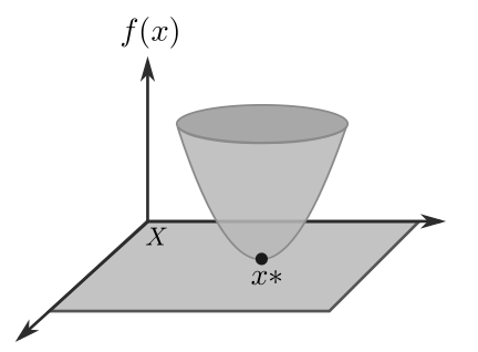
\begin{align} \label{eqn:Xargmin}
X^* &= \arg \min_{\vec{x} \in X} f(\vec{x}) \\ \nonumber
&= \{ \vec{x}^* \in X \ : \ f(\vec{x}^*) \leq f( \vec{x} ), \
%
\forall
%
\vec{x} \in X \}, \end{align}

where a bounded below function $f$ , i.e., $f(x^*) > -\infty$ is called objective function. $X$ is a $D$-dimensional parameter space, usually $X \subset \mathbb{R}^D$ is the domain for $\vec{x}$ representing constraints on allowable values for $\vec{x}$.

After the above description, a general single-objective BO problem with single-objective functions at both levels can be defined as follows:

Definition (Bilevel Optimization Problem) The 5-tuple $(F, \ f, \ X, \ Y, \ \mathbb{R} )$ is called bilevel problem if the the upper-level/leader’s objective function $F: X \times Y \to \mathbb{R}$ and the lower-level/follower’s objective function $f: X \times Y \to \mathbb{R}$. Then, the optimization process is formulated as follows:

Minimize:

\begin{equation}
F(\vec{x},\ \vec{y}) \text{ with } \ \vec{x} \in X , \ \vec{y} \in Y
\label{eqn:minF1}\end{equation}

subject to:

\begin{align} \label{eqn:y-arg} & \vec{y} \in \arg \min \{ f(\vec{x}, \vec{z}) \ : \vec{z} \in Y \}\\ \label{eqn:G} \end{align}

---

Note that, for simplicity, equality constraints were not considered in the definition above.

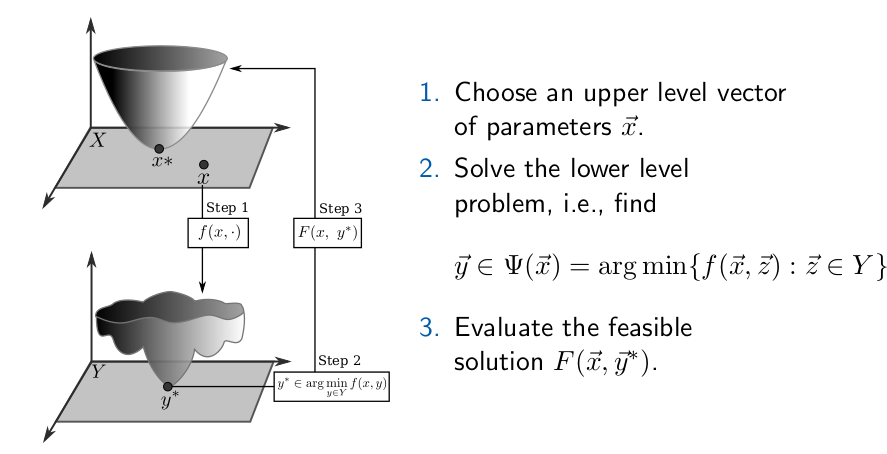
The figure below shows a schematic procedure to evaluate a solution in bi-level optimization problems.

In 1985, Jeroslow probed that linear bilevel optimization problems are NP-hard. After that, Hansen et al. showed that some BO problems are strongly NP-hard, since evaluating a solution in a bilinear programming problem is also NP-hard.

Example

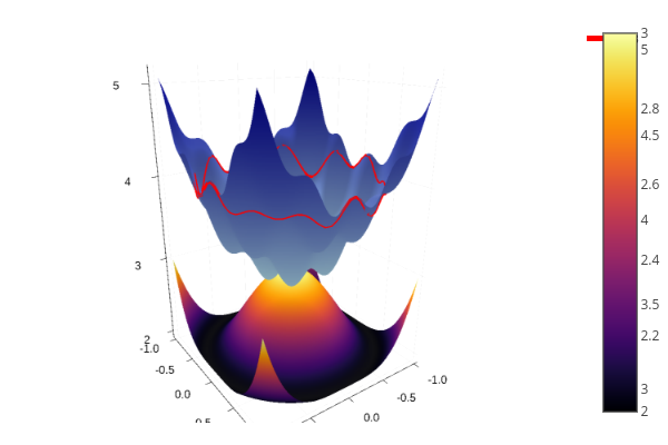
Consider the following bilevel problem:

Minimize:
$$
F(x, y) = x^2 + 0.1\cos(4\pi x) + y^2 + 0.1\sin(4\pi y)
$$

Subject to:
$$
y \in \arg \min \{ f(x, z) = (x^2 + z^2 -1)^2 \ : \ z\in Y \}
$$

Feasible Region

Th search space is defined over $X = Y = [0,1]$ and the feasible region is:

\begin{align*}
\{ (x, y)\in X \times Y \ : \ x^2+y^2 = 1 \}
&= \{ (x, \pm \sqrt{1 – x}) \ : \ x \in X \} \\
&= \{ (\cos(\theta),\ \sin(\theta)) \ : \ \theta \in [0, 2\pi) \}
\end{align*}