A Physics-Inspired Algorithm for Bilevel Optimization

1. Introduction

A new kind of optimization problem has been gaining interest by researchers in recent years. That problem was introduced in 1934 by Von Stackelberg in [1] and it is known nowadays as the Bilevel Optimization (BO) problem. A BO problem can be unconstrained, constrained, single and/or multi-objective, continuous and/or discrete, etc. but in any type it contains a nested optimization problem as a constraint [1]. Such introduced hierarchical structure can be useful to model decision-making processes, where a leader(upper level authority) optimizes their goals restricted to optimal decisions/solutions given by a follower (lower level authority) [1].

In order to formally introduce BO problems, we start by stating the traditional optimization problem. It is well known that, without loss of generality, an optimization problem can be defined as finding the set:

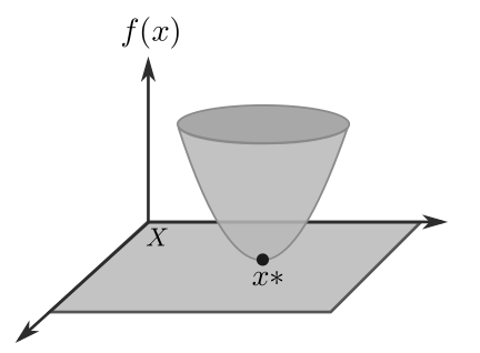
\begin{align} \label{eqn:Xargmin} X^* &= \arg \min_{\vec{x} \in X} f(\vec{x}) \\ \nonumber &= \{ \vec{x}^* \in X \ : \ f(\vec{x}^*) \leq f( \vec{x} ), \ \forall \vec{x} \in X \}, \end{align}

where a bounded below function $f$ , i.e., $f(x^*) > -\infty$ is called objective function. $X$ is a $D$-dimensional parameter space, usually $X \subset \mathbb{R}^D$ is the domain for $\vec{x}$ representing constraints on allowable values for $\vec{x}$. Eq. eqn:Xargmin may be read as: $X^*$ is the set of values (arguments) $\vec{x} = \vec{x}^*$ that minimizes $f(\vec{x})$ subject to $X^*$ (see Figure 1).

An optimization problem is solved only when a global minimum is found. However, global minimum are, in general, difficult to find. Therefore, in practice, we often have to find at least a local minimum [1].

After the above definitions, a general single-objective BO problem with single-objective functions at both levels can be defined as follows [1]:

Minimize

\begin{equation} F(\vec{x},\ \vec{y}) \ \ \vec{x} \in X , \ \vec{y} \in Y \label{eqn:minF1} \end{equation}
subject to:
\begin{align} \label{eqn:y-arg} &\vec{y} \in \arg \min \{ f(\vec{x}, \vec{y}) \ : \ g_j(\vec{x}, \vec{y}) \leq 0, \ j = 1,\ldots, J \}\\ &G_k(\vec{x}, \vec{y}) \leq 0, \ k = 1,\ldots,K \label{eqn:G} \end{align}

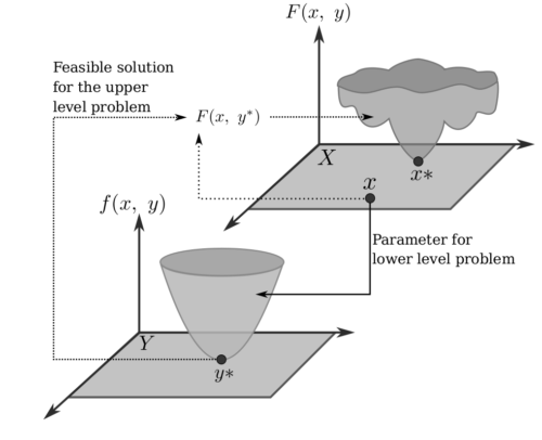
where $F: X \times Y \to \mathbb{R}$ and $f: X \times Y \to \mathbb{R}$ are the upper-level objective function (leader) and lower-level objective function (follower), respectively. In this work, $X \subseteq \mathbb{R}^n$ and $Y \subseteq \mathbb{R}^m$ are considered. Here, $G$ and $g$ are the inequality constraints of the upper and lower levels, respectively. Figure 2 shows a schematic diagram of a BO problem.

In 1992, Hansen et al. probed that BO problems are (strongly) NP-hard because evaluating a solution in the simplest BO problem (unimodal linear programming at both levels) is also NP-hard [1]. Moreover, many real-world problems can be naturally modeled as BO problems [1], for example: taxation, border security problems, transportation problems, machine learning algorithms tuning, among others [1].

Due to the importance of BO, many authors have proposed different kind of solutions for those problems e.g. mathematical approaches (mathematical programming, Karush-Kuhn-Tucker condition for single-level reduction) [1], evolutionary computation (genetic algorithms, evolution strategies) and swarm intelligence (particle swarm optimization) [1].

In order to handle BO problems three strategies are identified: (1) nested, (2) single-level reduction and (3) penalty methods. Nested strategies can be effective but with a high computational cost when objective functions are expensive to calculate or when high-dimensionality is present. Single-level reduction is used to transform a BO problem into a single-level problem, usually via Karush-Kuhn-Tucker conditions for smooth lower level objective function. As a consequence, this strategy is restricted to differentiable functions [1]. Penalty methods transform a constrained method into an unconstrained optimization problem by adding some penalties controlled by using parameters. This strategy can be simple to understand but hard to calibrate particularly in large-scale problems [1].

From the literature review above mentioned, regarding population-based metaheuristics for BO problems, most research efforts are focused on evolutionary computation and swarm intelligence algorithms because they have been successfully applied to solve single-level optimization problems. On the other hand, in recent years, physics-inspired algorithms have become popular to solve complex optimization problems and they have provided a competitive performance when solving single-level optimization problems [1].

This is the main motivation of this research work, where a first proposal of a physics-inspired algorithm, originally designed for global optimization [1], is now presented to deal with BO problems. Here, an unconstrained nested scheme is considered.

Our approach is called Bilevel Centers Algorithm (BCA) and it is based on the center of mass concept [1]. Without loss of generality, we assume a maximization problem for non-negative functions $f$ and $F$ for lower and upper objective functions, respectively. The center of mass concept is used in both levels, in order to generate new biased directions towards promising/feasible regions of the search space.

2. Lower Level Optimizer

The center of mass is the unique point $\vec{c}$ at the center of a mass distribution $U = \{\vec{u}_1,\; \vec{u}_2 , \ldots , \vec{u}_K \}$ in a space that has the property that the weighted sum of $K$ position vectors relative to this point is zero [1], as indicated in Eq. eqn:masscenter:

\begin{equation} \sum_{i = 1}^K m(\vec{u}_i) (\vec{u}_i – \vec{c}) = 0, \text{ implies } \vec{c} = \dfrac{1}{M} \sum_{i = 1}^K m(\vec{u}_i) \vec{u}_i, \label{eqn:masscenter} \end{equation}

where $m(\vec{u}_i)$ is the mass of $\vec{u}_i$ and $M$ is the sum of the masses of vectors in $U$. Here, $m$ is a non-negative function.

Thus, the lower level optimizer works as follows: for each solution $\vec{y}_i $ in the population $P = \{ \vec{y}_1,\ \vec{y}_2, \ \ldots, \ \vec{y}_{N} \} $ of $N$ solutions in $Y$, we generate $U_i \subset P $ with $K$ different solutions such that

$$ \bigcup_{i=1}^N U_i = P. $$

Next, from $U_i$ the center of mass $\vec{c}_i$ is computed by using Eq. eqn:masscenter considering $m(\vec{u}) = f(\vec{p}, \vec{u})$, where $\vec{p}$ is given by the upper level optimizer. After that, the worst element $\vec{u}_{\text{worst}}$ in $U_i$ is selected according to the following rule:

$$ \vec{u}_{\text{worst}} \in \arg \min \{f(\vec{p}, \ \vec{u} ) \ : \ \vec{u} \in U_i \}. $$

Now, we are able to generate a direction to locate a new solution $ \vec{q}_i$ using the already generated center of mass $\vec{c}_i$, the current solution $\vec{y}_i$ and the worst solution $\vec{u}_{\text{worst}}$ by using Eq. eqn:vcu2:

\begin{equation} \vec{q}_i = \vec{y}_i + \eta _{i} ( \vec{c}_i – \vec{u}_{ \text{worst} } ) , \label{eqn:vcu2} \end{equation}

Due to this stochastic strategy, this variation operator can help the exploration-exploitation process to avoid premature convergence because it combines the center of mass as an attractor to promising regions of the search space but using the position of the worst solution as a reference to get far away from it [1]. The replacement operator works as follows: if $\vec{q}_i$ is better than $\vec{y}_i$, then the worst element in $P$ is replaced by $\vec{q}_i$.

A linear reduction of the population size (deleting the worst elements) is applied. The initial population size is $ N(0) = K*D$ and the final population size $N(T) = 2*K$ (for successfully generating the center of mass). Thus, the population size over time is as in Eq. eqn:redpop: \begin{equation} N(t) = KD – \dfrac{(KD – 2K) t}{T} = K \left( D – \dfrac{(D – 2) t}{T} \right), \label{eqn:redpop} \end{equation} where $t = 0,1,2,\ldots,T$ and $T$ is the maximum number of iterations.

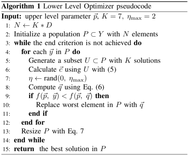
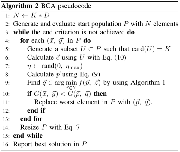
The procedure for the implementation of the lower level optimizer is detailed in Algorithm 3.

3. BCA

Here, BCA is presented as the upper lower level optimizer. We start describing the variation operator of BCA and its properties. Let $F$ and $f$ be defined as in Eq. (eqn:minF1) and Eq. (eqn:y-arg), respectively. Without loss of generality we can assume that both $F$ and $f$ are non-negative and we want to maximize them. Hence, the population for a BO problem can be defined as in Eq. eqn:ECApop: \begin{equation} P = \{ (\vec{x}_1,\; \vec{y}_1), \ (\vec{x}_2,\; \vec{y}_2), \ldots, (\vec{x}_N,\; \vec{y}_N) \} \subset X \times Y, \label{eqn:ECApop} \end{equation} where $\vec{y}_i \in \arg \min \{ f(\vec{x}_i, \ \vec{z}) \ : \ \vec{z} \in Y \}$ for $i = 1,\ldots,N$. Here, $\vec{x}_i$ is generated at random with uniform distribution.

3.1. Algorithm Description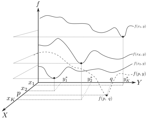

Now, we are able to describe the BCA procedure: for each iteration and each solution $(\vec{x}_i,\; \vec{y}_i) \in P$, a new upper level parameter is generated using the formulation in Eq. eqn:vcu2F: \begin{equation} \vec{p}_i = \vec{x}_i + \eta _{i} ( \vec{c}_i – \vec{u}_{ \text{worst} } ), \label{eqn:vcu2F} \end{equation} where the $\vec{c}_i$ is the center of mass computed using: \begin{equation} \vec{c}_i = \dfrac{1} {W} \sum_{(x,y) \in U} Q(\vec{x},\ \vec{y}) \cdot \vec{x} , \hspace{0.5cm} W = \sum_{ (x,y) \in U} Q(\vec{x},\ \vec{y}), \label{eqn:centerF} \end{equation} where $Q(\vec{x},\ \vec{y}) = F(\vec{x},\ \vec{y}) + f(\vec{x},\ \vec{y})$, $U \subset P $ such that card$(U) = K$ and $\vec{u}_{ \text{worst}}$ is the first coordinate of the worst element in $U$, see Eq. eqn:uplev-worst.

\begin{equation} \vec{u}_{\text{worst}} \in \arg \min \{Q(\vec{u}, \ \vec{y} ) \ : \ \vec{u} \in U_i \} \label{eqn:uplev-worst} \end{equation}

Note that the function $Q(\vec{x},\ \vec{y})$ is used to translate the upper level population towards regions where $F$ is maximized while $f$ may control the bias to feasible solutions.

Finally, the new solution is given by $ (\vec{p}, \ \vec{q}) $ which may replace the worst solution in $ P $ if it is better than $(\vec{x}_i,\; \vec{y}_i)$. Here, $ \vec{q} = \arg \min _ {\vec{z} \in Y} f (\vec{p}, \ \vec{z}) $ obtained by applying Algorithm 3. Figure 4 shows a representation of BCA solution update.

The BCA approach requires the definition of three parameter values: $K$, $\eta_{\max}$ and the population size. Here, $K$ is useful to handle the multi-modality, i.e., large $K$ values provide fast convergence to local optima (useful for unimodal functions). When $K$ takes small values, BCA favors an exploratory process. $\eta_{\max}$ mainly controls the exploratory process as the stepsize is controlled by this parameter. The parameter setting recommended by preliminary experiments is $K = 7$ and $\eta_{\max} = 2$.

BCA is summarized in Algorithm 5. This proposed algorithm was used to solve a set of eight test problems to assess the performance of BO algorithms, known as SMD problems. Those test problems are described in [1].

4. Experiments and Discussion

The configuration used in BCA for the experiments performed was as follows: The number of Function Evaluations (NFEs) was fixed for the upper level: $500D_{UL} = 2500$, and the lower level: $500D_{UL}*500D_{LL} = 6,250,000$ total NFEs for both levels. The remaining parameters were set as follows:

• Upper level dimension $D_{UL} = 5$
• Lower level dimension $D_{LL} = 5$
• Upper level population size $K*D_{UL}$
• Lower level population size $K*D_{LL}$
• $K = 7$
• $\eta_{\max} = 2$
• Stop condition: BCA stopped when the accuracy ($1\times 10^{-4}$) or the maximum NFEs allowed was reached.

BCA was compared against BLEAQ which is a state-of-the-art evolutionary algorithm for BO problems [1]. BLEAQ is based on quadratic approximations of optimal lower level variables with respect to the upper level variables. Such strategy lets BLEAQ to reduce the NFEs having competitive results. BLEAQ was run with the parameters suggested by the authors [1] and the stop criteria was maintained but accuracy was set at $1\times 10^{-4}$ as in BCA. Both algorithms were used to solve independently 31 times each test problem.

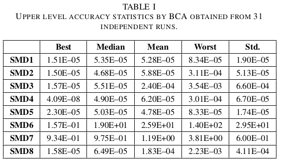
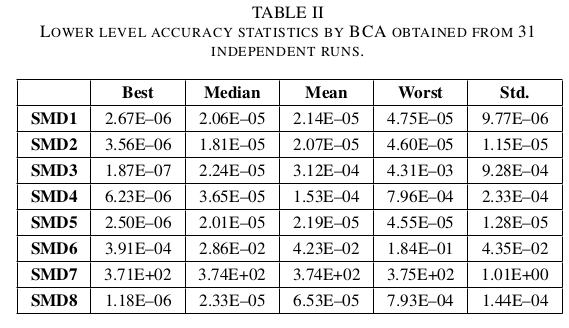
Tables 6 and 7 show the statistical results of the accuracy values obtained by the proposed BCA in the two levels of each BO test problem. Moreover, the best, median, mean, worst and standard deviation values of the NFEs required to solve each BO test problem using BCA are given in Table 9 and tab:ll-fes for each level, respectively. Tables tab:ul-comparative-fes and 11 compare the median accuracy and NFEs at the upper and lower levels required by BCA against those values obtained by BLEAQ. A result in boldface indicates the best value found.

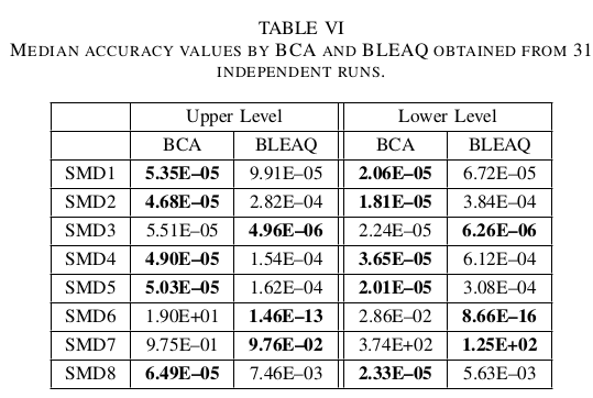
From Tables 6 and 7 it can be observed that BCA is able to consistently reach very competitive results in all test problems for both levels. Just problem SMD7 was difficult to solve by BCA.

A similar robust performance was observed by BCA in the upper level regarding NFEs as indicated in Table 9. In contrast, more variation in the number of NFEs was reported in Table tab:ll-fes for the lower level.

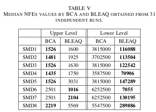
Regarding the comparison against the state-of-the-art algorithm, from Table 11 it can be concluded that BCA outperformed BLEAQ in five BO test problems in the upper level and also in five BO test problems in the lower level. Furthermore, BCA required less NFEs in the upper level of six BO test problems based on Table tab:ul-comparative-fes. However, BLEAQ clearly outperformed BCA in the number of lower level NFEs as indicated in the same Table tab:ul-comparative-fes.

Note that no statistical test was used to compare the algorithms, since the obtained values (from the objective functions) may not represent feasible solutions and that can be an unfair comparison of the performance of the algorithms.

5. Conclusions

This work presented the adaptation of a physics-inspired algorithm based on the center of mass (BCA) to solve bilevel optimization problems. Both levels used a similar variation operator based on the center of mass to find promising regions of the search space and a greedy replacement based on fitness. BCA is a simple algorithm which requires just three parameters to be fine-tuned by the user (the population size, the size of the subset to compute the center of mass and the stepsize for the variation operator). Eight test problems were solved to assess the performance of the proposed algorithm in terms of upper/lower level accuracy and function evaluations compared against a state-of-the-art evolutionary algorithm for BO. The overall results suggest that BCA was able to provide competitive results in terms of accuracy compared to those obtained by BLEAQ even requiring less evaluations in the upper level. However BLEAQ outperformed BCA with respect to the number of evaluations required at the lower level. Additional resources (code, tutorials, etc.) about bilevel optimization can be found at http://bi-level.org.

Full Paper and Citation

@inproceedings{mejia2018physics,
  title={A Physics-Inspired Algorithm for Bilevel optimization},
  author={Mej{\'\i}a-de-Dios, Jesus-Adolfo and Mezura-Montes, Efr{\'e}n},
  booktitle={2018 IEEE International Autumn Meeting on Power, Electronics and Computing (ROPEC)},
  pages={1--6},
  year={2018},
  organization={IEEE}
}