Tutorial: Bilevel Optimization Without Tears

This tutorial offers a gentle introduction to bilevel optimization (BO) by using practical examples but highlighting the main differences between BO and other traditional optimization tasks such as global optimization, constrained optimization and multi-, many-objective optimization. A bird’s-eye view describing mathematical-programming-based and also metaheuristic-based approaches is considered as well. Finally, an online resource will be provided to the attendees, so they can write and solve their own BO problem.

This tutorial was presented at the International Workshop on Numerical and Evolutionary Optimization NEO 2020

by Jesús-Adolfo Mejía-de Dios & Efrén Mezura-Montes

Optimization

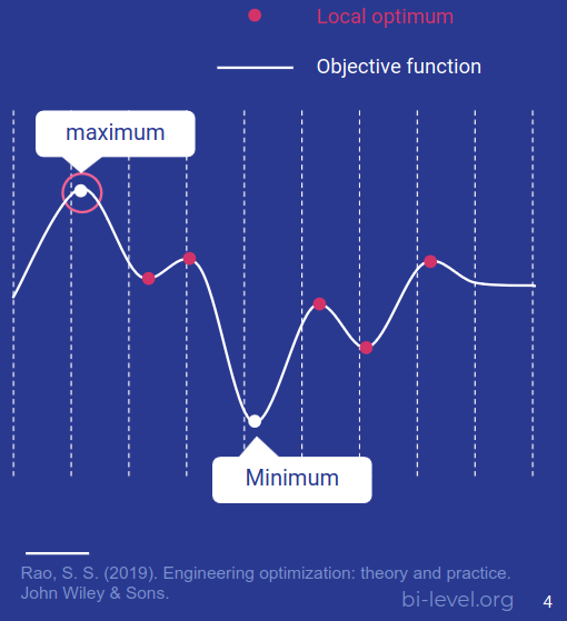
Optimization refers to the process of finding the best possible solution among a set of alternatives for a specific problem or objective. It involves maximizing or minimizing a function (a.k.a. objective function, target function or fitness function), and satisfying constraint functions.

Optimization can be used in a wide range of domains, including mathematics, engineering, economics, computer science, and more. The goal is to determine the most efficient or optimal solution that meets the desired criteria, whether it’s maximizing profits, minimizing costs, improving performance, or achieving the best outcome within the given constraints.

Solution techniques include algorithms and mathematical models to explore the solution space and iteratively refine the options until an optimal solution is found.

Bilevel Optimization

Bilevel optimization is a type of optimization problem that involves two levels containing an optimization problem each.

One optimization problem is nested within the other optimization problem.

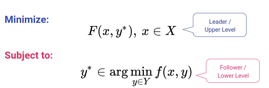
The upper-level problem, also known as the leader problem, aims to optimize an objective function while considering the solutions of the lower-level problem, known as the follower problem. The follower’s decisions are influenced by the decisions made by the leader problem.

An upper level authority takes a decision subject to an optimal response from a lower level authority

Zhang, G., et al (2015). Multi-level decision making. New York: Springer.

Bilevel optimization is commonly used in various areas, such as economics, engineering, and decision-making, where the interaction and interdependence between two optimization levels need to be considered to find the best overall solution.

Bilevel optimization: Dummy example

A guy finds the best way to escape, subject to the optimal path (to the guy’s position) planned by the chickens (see figure below).

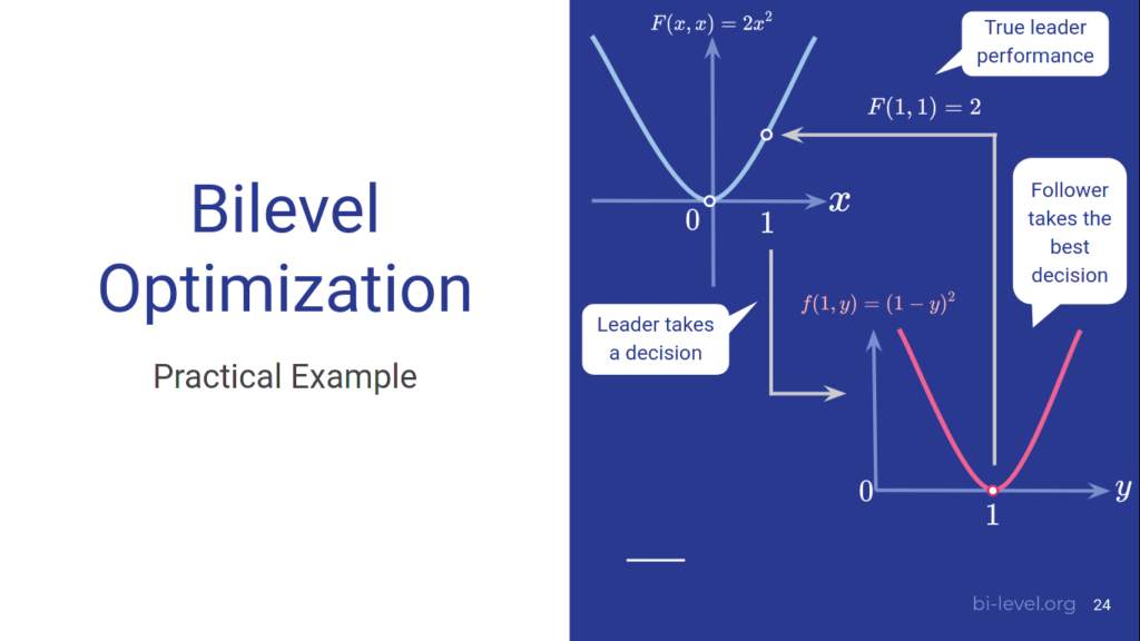
Let’s analyze this peculiar problem level by level. Here, the leader is the guy, who needs to escape from the chickens. As you may note, the guy takes a decision x.

Once, the leader takes a decision x, the follower (chicken) needs to update her/his decision y considering the decision given by the leader.

Definition of a Bilevel Optimization Problem

Bilevel optimization is formally defined as a mathematical programming model where an upper-level problem seeks to optimize an objective function, subject to constraints that are influenced by the solutions of a lower-level problem, which is also an optimization problem.

The nested scheme in bilevel optimization refers to the hierarchical structure where one optimization problem is embedded within another, with the upper-level problem influencing the lower-level problem.

Solution of a Bilevel Optimization Problem

A bilevel solution, a pair (x, y) of decision variables that satisfies the constraints and objectives of both the upper-level and lower-level optimization problems. It represents a feasible solution that accounts for the interdependence between the two levels, i.e., if x is an upper-level decision variable, y corresponds to an optimal solution from the lower level.

1. Feasible solution: A feasible solution refers to a set of decision variables that satisfies both the constraints of the upper-level and lower-level problems.
2. Inducible region: The inducible region contains all the feasible solution of a bilevel problem.
3. Optimal feasible solution: A feasible optimal solution refers to a set of decision variables (x, y) that achieves the best overall objective value while satisfying the constraints of both the upper-level and lower-level problems. That is, are those solutions in the inducible region optimizing the upper-level objective function.

How to know if my problem requires bilevel structure?

If your problem has all the following elements, you probably need a bilevel optimization model:

• An evident hierarchical structure involving
• Two objective functions, each defined on
• Two separate search spaces (domains).

Although there are more items that are required, the ones listed above are necessary conditions.

Final Remark

Studying bilevel optimization can provide valuable insights into complex systems, economics, engineering, and decision-making scenarios. By exploring the interplay between upper-level and lower-level optimization problems, you can gain a deeper understanding of how different variables and constraints influence each other, leading to more informed and optimal solutions.